Part 4 : Similarity Network Fusion with Graph Convolutional Networks

In the previous notebook we trained a Graph Convolutional Network on two similarity matrices. We found that when our network is bad, our performance is bad. When we have a more informative network we can improve this performance.

Neither of our networks were more expressive than performing a basic linear regression however. We are not fully leveraging the power of neworks, in particular their flexibility.

In this notebook we will use the Similarity Network Fusion (SNF) algorithm to integrate a second modality.

In this part we will :

• Create a second patient similarity network

• Train a quick GCN on this modality to test it’s accuracy

• Perform SNF to integrate our two modalities

• Retrain a GCN on the combined network

Import Functions and Packages

import pickle
import pandas as pd
import numpy as np
import networkx as nx
import matplotlib.pyplot as plt
from palettable import wesanderson
import snf
import sys
sys.path.insert(0 , '/tutorial/')
from functions import *
from sklearn.model_selection import train_test_split
import os
os.environ["DGLBACKEND"] = "pytorch"
import dgl
import torch

Import and Process Generation Scotland Data

with open('/data/intermediate/GCN_Data.pkl' , 'rb') as file : 
    loaded_data = pd.read_pickle(file)

phenotypes = loaded_data['phenotypes']

Create Patient Similarity Network for Second Modality

NOTE : Creating second modality of time since last cigarette. This will be highly correlated with the outcome of smoking or not however, we want to use this as an exemplar for SNF + GNN’s

from sklearn.preprocessing import MinMaxScaler

def time_since_last_smoked(row) : 
    if row['pack_years'] == 0 : 
        return row['age']
    else :
        if row.isna()['stopped'] :
            return 0
        else : 
            return row['stopped']
        
phenotypes['time_since_last_smoked'] = phenotypes.apply(time_since_last_smoked , axis =1)

'''
#################################################
                YOUR CODE HERE
#################################################
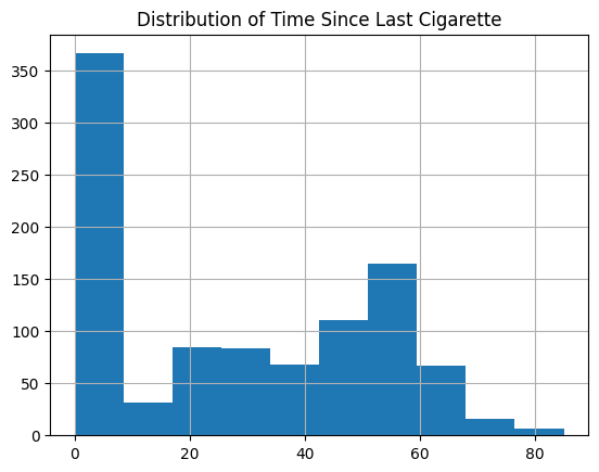
Plot the distribution of the Time Since Last Cigarette Phenotype
'''

phenotypes['time_since_last_smoked'].hist()
plt.title('Distribution of Time Since Last Cigarette')
plt.show()

'''
#################################################
                YOUR CODE HERE
#################################################
Here we will infer a similarity between patients based on their time since last cigarette
In order to calculate this we will 

1. Scale the data using the MinMaxScaler
2. Create an empty nxn dataframe of zeros with the patients on the index and columns
3. Fill the dataframe on the euclidean distance between each patients time_since_last_smoked 

'''

scaler = MinMaxScaler()
scaled_time = scaler.fit_transform(phenotypes[['time_since_last_smoked']]).reshape(1,-1)[0]

n = len(scaled_time)

# Create a DataFrame filled with zeros
df = pd.DataFrame(np.zeros((n, n)) , columns=phenotypes.index , index=phenotypes.index)

# Fill the DataFrame with the differences
for i, integer in enumerate(scaled_time):
    df.iloc[i, :] = 1 - np.abs(np.array(scaled_time) - integer)

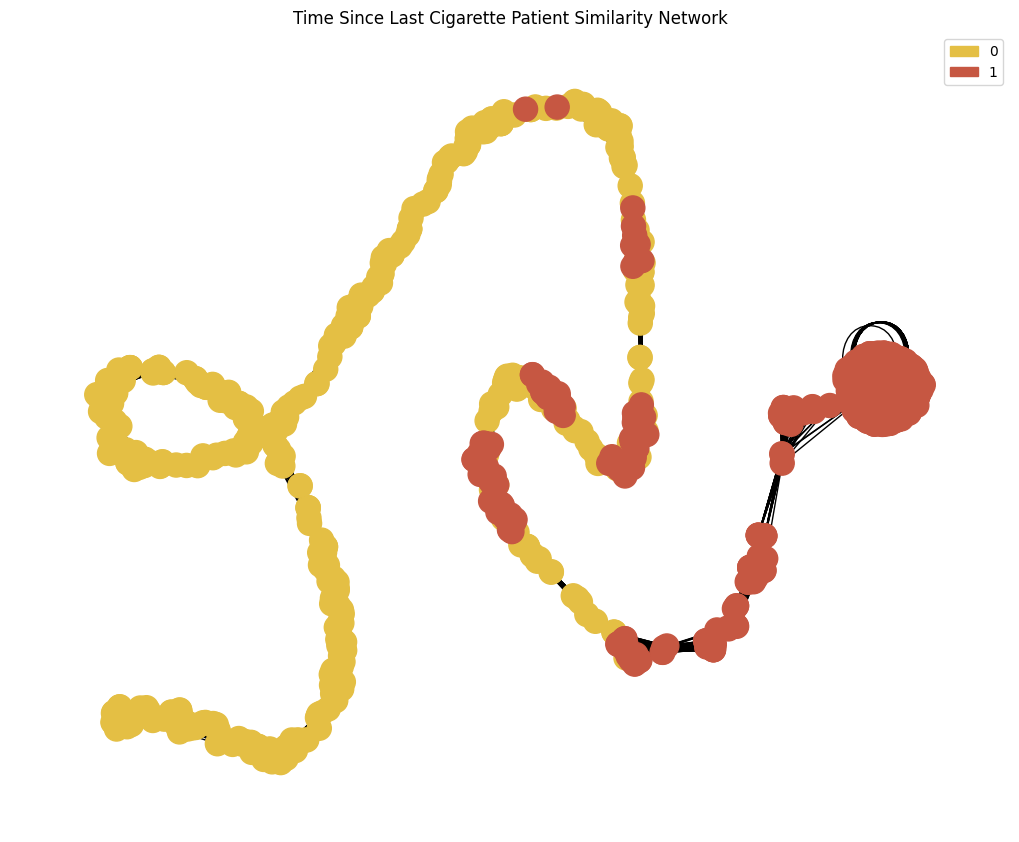
Plot the Time Since Last Smoked Network

node_colour = phenotypes['Smoking'].astype('category').cat.set_categories(wesanderson.FantasticFox2_5.hex_colors , rename=True)

print(f"{phenotypes['Smoking'].astype('category').cat.categories[0]} : 0 \n{phenotypes['Smoking'].astype('category').cat.categories[1]} : 1")

G_time_to_smoke = plot_knn_network(df , 25 , phenotypes['Smoking'] , node_colours=node_colour)
plt.title('Time Since Last Cigarette Patient Similarity Network')
legend_handles = gen_graph_legend(node_colour , G_time_to_smoke , 'label')
plt.legend(handles = legend_handles)
plt.show()

Non-Smoker : 0 
Smoker : 1

Train GCN on second modality for comparison of performance

Here we will re-use the code from the previous section, specifically the train and evaluate functions.

g = dgl.from_networkx(G_time_to_smoke , node_attrs=['idx' , 'label']) # Convert networkx graph to dgl graph
g.ndata['feat'] = torch.Tensor(loaded_data['Feat'].iloc[g.ndata['idx'].numpy()].values) # Add node features to graph

device = ('cuda' if torch.cuda.is_available() else 'cpu') # Use GPU if available

g = g.to(device) # Move graph to device

node_subjects = phenotypes['Smoking'].iloc[g.ndata['idx'].detach().cpu().numpy()].reset_index(drop=True) # Get node target labels from meta data
node_subjects.name = 'Smoking'

train_tmp_index , test_index = train_test_split(                 # Split data into temporary training and testing sets
    node_subjects.index, train_size=0.6, stratify=node_subjects
    )
train_index , val_index = train_test_split(                       # Split temporary training data into training and validation sets
    train_tmp_index, train_size=0.8, stratify=node_subjects.loc[train_tmp_index]
    )

GCN_input_shapes = g.ndata['feat'].shape[1] # Get input shape for GCN

labels = F.one_hot(g.ndata['label'].to(torch.int64)) #  One hot encode labels

output_metrics = []
logits = np.array([])
labels_all = np.array([])

model = GCN(GCN_input_shapes , [128], len(node_subjects.unique())).to(device)  # Create GCN model
print(model)
print(g)

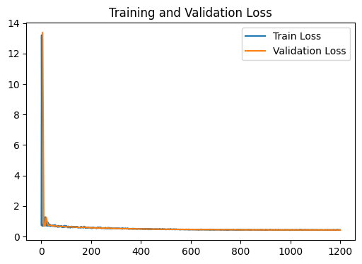
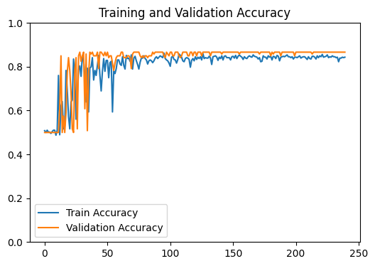
loss_plot = train(g, g.ndata['feat'] , train_index , val_index , device ,  model , labels , 1200 , 1e-3) # Train model
plt.show()

test_output_metrics = evaluate(test_index , device , g , g.ndata['feat'] , model , labels ) # Evaluate model on test set

print(
    "GNN Model | Test Accuracy = {:.4f} | F1 = {:.4f} |".format(
     test_output_metrics[1] , test_output_metrics[2] )
)

GCN(
  (gcnlayers): ModuleList(
    (0): GraphConv(in=23676, out=128, normalization=both, activation=None)
    (1): GraphConv(in=128, out=2, normalization=both, activation=None)
  )
  (batch_norms): ModuleList(
    (0): BatchNorm1d(128, eps=1e-05, momentum=0.1, affine=True, track_running_stats=True)
  )
  (drop): Dropout(p=0.05, inplace=False)
)
Graph(num_nodes=1000, num_edges=34843,
      ndata_schemes={'idx': Scheme(shape=(), dtype=torch.int64), 'label': Scheme(shape=(), dtype=torch.int8), 'feat': Scheme(shape=(23676,), dtype=torch.float32)}
      edata_schemes={})

GNN Model | Test Accuracy = 0.8875 | F1 = 0.8659 |

Similarity Network Fusion (SNF)

We will once again implement SNF from the paper by Wang et al.

We will implement it using the python package snfpy

'''
#################################################
                YOUR CODE HERE
#################################################

We need to create a list with all the graphs we want to include in SNF.
In this section you will need to : 
    1. Convert the graphs into pandas adjacency matrices hint : use nx.to_pandas_adjacency()
    2. Append the adjacency matrices to the list.

'''
G_DNAm = loaded_data['PSN_EWAS']
full_graphs = []

for graph in [G_time_to_smoke , G_DNAm] : 
    graph = nx.to_pandas_adjacency(graph)
    
    full_graphs.append(graph)

'''
#################################################
                YOUR CODE HERE
#################################################

Here we will perform SNF to fuse our two modalities of data.

1. Use the SNF function from the snf package to fuse the graphs in full_graphs. Use k = 25 and t = 10.
2. Convert the numpy array output from the SNF function to a pandas DataFrame with the index and columns as the patient IDs.

'''
adj = snf.snf(full_graphs , K = 25 , t = 10)

adj_snf = pd.DataFrame(data=adj , index=phenotypes.index , columns=phenotypes.index) 

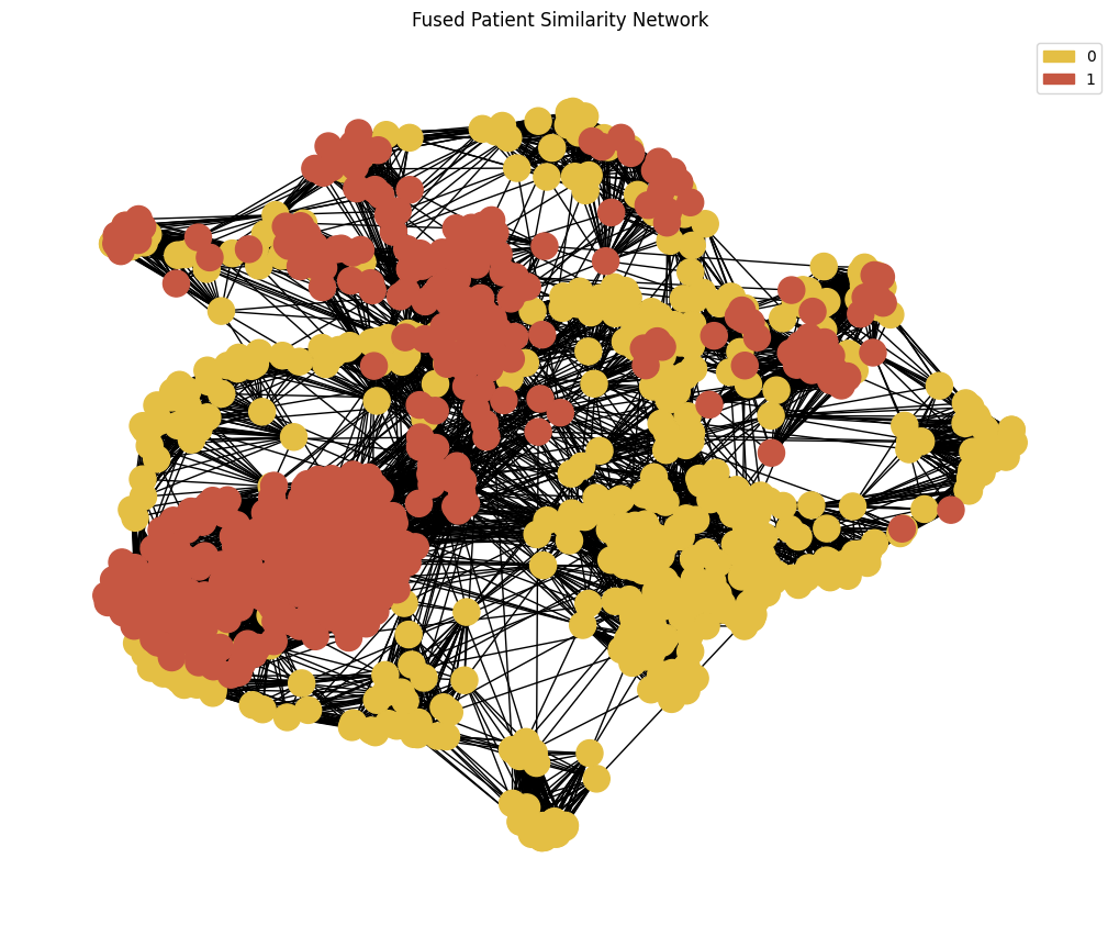
Note that SNF returns a fully connected graph. We will sparsify the edges by performing KNN based on the similarity weights from SNF

We have provided this functionality previously in the plot_knn_network function

node_colour = phenotypes.loc[adj_snf.index]['Smoking'].astype('category').cat.set_categories(wesanderson.FantasticFox2_5.hex_colors , rename=True) # Set node colours

G = plot_knn_network(adj_snf, k , phenotypes['Smoking'] , node_colours=node_colour)  # Plot the fused network and get back networkx graph
plt.title('Fused Patient Similarity Network')
legend_handles = gen_graph_legend(node_colour , G , 'label') # Generate legend
plt.legend(handles = legend_handles)
plt.show()

GCN on SNF network

We now have fused our graphs into a single patient similarity network and we are ready to learn from this.

Again we will re-use the code from the previous part but changing our graph to the the SNF graph created above.

g = dgl.from_networkx(G , node_attrs=['idx' , 'label']) # Convert networkx graph to dgl graph
g.ndata['feat'] = torch.Tensor(loaded_data['Feat'].iloc[g.ndata['idx'].numpy()].values) # Add node features to graph

device = ('cuda' if torch.cuda.is_available() else 'cpu') # Use GPU if available

g = g.to(device) # Move graph to device

node_subjects = phenotypes['Smoking'].iloc[g.ndata['idx'].detach().cpu().numpy()].reset_index(drop=True) # Get node target labels from meta data
node_subjects.name = 'Smoking'

train_tmp_index , test_index = train_test_split(                # Split data into temporary training and testing sets
    node_subjects.index, train_size=0.6, stratify=node_subjects
    )
train_index , val_index = train_test_split(                     # Split temporary training data into training and validation sets
    train_tmp_index, train_size=0.8, stratify=node_subjects.loc[train_tmp_index]
    )

GCN_input_shapes = g.ndata['feat'].shape[1]  # Get input shape for GCN

labels = F.one_hot(g.ndata['label'].to(torch.int64)) # One hot encode labels

output_metrics = []
logits = np.array([])
labels_all = np.array([])

model = GCN(GCN_input_shapes , [128], len(node_subjects.unique())).to(device)  # Create GCN model
print(model)
print(g)

loss_plot = train(g, g.ndata['feat'] , train_index , val_index , device ,  model , labels , 1200 , 1e-3) # Train model
plt.show()

test_output_metrics = evaluate(test_index , device , g , g.ndata['feat'] , model , labels ) # Evaluate model on test set

print(
    "GNN Model | Test Accuracy = {:.4f} | F1 = {:.4f} |".format(
     test_output_metrics[1] , test_output_metrics[2] )
)

GCN(
  (gcnlayers): ModuleList(
    (0): GraphConv(in=23676, out=128, normalization=both, activation=None)
    (1): GraphConv(in=128, out=2, normalization=both, activation=None)
  )
  (batch_norms): ModuleList(
    (0): BatchNorm1d(128, eps=1e-05, momentum=0.1, affine=True, track_running_stats=True)
  )
  (drop): Dropout(p=0.05, inplace=False)
)
Graph(num_nodes=1000, num_edges=29970,
      ndata_schemes={'idx': Scheme(shape=(), dtype=torch.int64), 'label': Scheme(shape=(), dtype=torch.int8), 'feat': Scheme(shape=(23676,), dtype=torch.float32)}
      edata_schemes={})

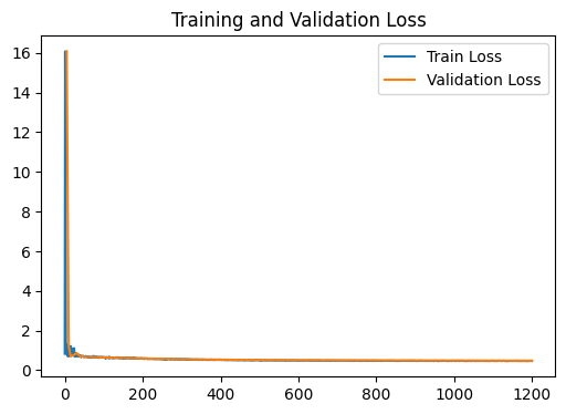
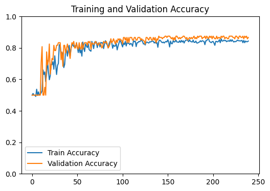
GNN Model | Test Accuracy = 0.8600 | F1 = 0.8340 |