Part 3 : Smoking Network Classification using Graph Convolutional Networks#
In this part we will work with a Graph Convolutional Network (GCN).
In the previous part we formulated a task to predict whether individuals in the Generation Scotland Dataset have ever smoked.
We generated a patient similarity network from CpG sites which are known to be associated with smoking. We will also work with the patient similarity network generated in section 1.
In this part we postulate that individuals who have previously smoked will share similar epigenetic markers which we can learn from. We will now highlight the difference between our two networks to see if we can learn from them
In this part we will be :
Working with Deep Graph Library
Building a GCN
Training a GCN
Comparing the performance of PSN’s
Comparing the performance of GCN to simple linear regression
Import Functions and Packages #
import pickle
import pandas as pd
import numpy as np
import networkx as nx
import matplotlib.pyplot as plt
import sys
sys.path.insert(0 , '/tutorial/')
from functions import *
Load Data and Network #
# Load the data using pickle
with open('/data/intermediate/GCN_Data.pkl' , 'rb') as file :
    loaded_data = pd.read_pickle(file)
Working with Deep Graph Library#
import os
os.environ["DGLBACKEND"] = "pytorch"
import dgl
import torch

'''
#################################################
                YOUR CODE HERE
#################################################
Create a DGL graph from the networkx graph

Add the features to the nodes, ensuring the order of the
features matches the order of the nodes.

Note : DGL only accepts torch.Tensors as feature attributes
'''

g = dgl.from_networkx(loaded_data['PSN_EWAS'] , node_attrs=['idx' , 'label']) # Create a DGL graph from the networkx graph
g.ndata['feat'] = torch.Tensor(loaded_data['Feat'].iloc[g.ndata['idx'].numpy()].values) # Add the features to the nodes
# Sanity Check that our graph is preserved
phenotypes = loaded_data['phenotypes'] # Load the phenotypes

node_0 = phenotypes.iloc[g.ndata['idx'].numpy()].iloc[0] # Get the idx of the first node of the dgl graph

node_0_edges = []
for e1 , e2 in loaded_data['PSN_EWAS'].edges(node_0.name) :  # Get the edges of this node in the networkx graph
    node_0_edges.append(e2)

'''
###########################################################################
Note : DGL will reorder the nodes if integers are present in the node name
###########################################################################
'''

sorted(list(phenotypes.iloc[g.ndata['idx'].numpy()].iloc[g.out_edges(0)[1].numpy()].index)) == sorted(node_0_edges) # Check if the edges match between the networkx and dgl graph
True
Graph Convolutional Network #
Here we will specify the layers of the GCN model using the GraphConv class from DGL.
See Object Oriented Programming for more information on building classes in python.
See GraphConv for more documentation on the class.
import torch.nn as nn
import torch.nn.functional as F
from dgl.nn import GraphConv

class GCN(nn.Module):
    def __init__(self, input_dim,  hidden_feats, num_classes):

        super().__init__()

        self.gcnlayers = nn.ModuleList()
        self.drop = nn.Dropout(0.1)
        '''
        #################################################
                       YOUR CODE HERE
        #################################################
        The GraphConv class takes in the following arguments:
            1. input_dim : The number of input features
            2. output_dim : The number of output features
            3. activation : The activation function to be used after the layer (we will stick to the default which is None)

        We will create a list of GraphConv layers with the following dimensions:
            1. input_dim -> hidden_feats[0]
            2. hidden_feats[0] -> hidden_feats[1]
            3. hidden_feats[1] -> num_classes

        Where hidden_feats is a list of the number of hidden features in each layer which we will specify later
        '''
        self.gcnlayers.extend([
            GraphConv(input_dim , hidden_feats[0]),
            GraphConv(hidden_feats[0] , hidden_feats[1]),
            GraphConv(hidden_feats[1] , num_classes)
        ])

    def forward(self, g, h):
        # list of hidden representation at each layer (including the input layer)

        '''
        #################################################
                       YOUR CODE HERE
        #################################################

        Here we will define the forward pass of the GCN model.

        The forward pass will consist of the following steps:
            1. Pass the input features through the first GraphConv layer
            2. Apply dropout on the output of the first layer & ReLU activation function hint use F.relu
            3. Pass the output of the first layer through the second GraphConv layer
            4. Apply dropout on the output of the first layer & ReLU activation function hint use F.relu
            5. Pass the output of the second layer through the third GraphConv layer
            6. Return the output of the third layer
        '''

        h = self.gcnlayers[0](g , h)
        h = F.relu(self.drop(h))
        h = self.gcnlayers[1](g , h)
        h = F.relu(self.drop(h))
        h = self.gcnlayers[2](g , h)

        return h
Training & Evaluation #
We need to define training and evaluation functions for our GCN model. The code provided follows the outline defined in Chapter 6 of Hamilton’s book for training GNN’s.
The code below is fully operational and provided for practical demonstration. Similar examples of GNN training functions are provided by DGL in their Blitz Introduction
In these functions we implement Cross Entropy Loss for multi-class classification. We use the Adam Optimizer to update the model parameters and we use the StepLR function to decay the learning rate
import torch.optim as optim
import torch.nn as nn
import sklearn as sk
import seaborn as sns
from sklearn.metrics import precision_recall_curve , average_precision_score , recall_score ,  PrecisionRecallDisplay
from tqdm.notebook import tqdm
from sklearn.model_selection import train_test_split

def train(g, h, train_split , val_split , device ,  model , labels , epochs , lr):
    # loss function, optimizer and scheduler
    loss_fcn = nn.CrossEntropyLoss() # [Cross Entropy Loss for multi-class classification](https://pytorch.org/docs/stable/generated/torch.nn.CrossEntropyLoss.html)
    optimizer = optim.Adam(model.parameters(), lr=lr , weight_decay=1e-4) # Optimizer to update model parameters [Adam Optimizer](https://pytorch.org/docs/stable/optim.html#torch.optim.Adam)
    scheduler = optim.lr_scheduler.StepLR(optimizer, step_size=50, gamma=0.8) # Scheduler function to decay the learning rate [StepLR](https://pytorch.org/docs/stable/generated/torch.optim.lr_scheduler.StepLR.html)

    train_loss = []
    val_loss   = []
    train_acc  = []
    val_acc    = []

    # training loop
    epoch_progress = tqdm(total=epochs, desc='Loss : ', unit='epoch') # tqdm progress bar for epochs
    for epoch in range(epochs):
        model.train() # Set the model to training mode

        logits  = model(g, h) # Get the logits from the model. Logits are analagous to the node features estimates obtained during the karate club toy example

        loss = loss_fcn(logits[train_split], labels[train_split].float()) # Calculate the loss i.e. how far off the model is from the true labels
        train_loss.append(loss.item())

        optimizer.zero_grad() # Zero the gradients before backpropagation
        loss.backward() # Backpropagate the loss
        optimizer.step() # Update the model parameters based on the gradients

        scheduler.step() # Step the scheduler to decay the learning rate

        if (epoch % 5) == 0 :

            _, predicted = torch.max(logits[train_split], 1) # Get the predicted labels from the model
            _, true = torch.max(labels[train_split] , 1) # Get the true labels
            train_acc.append((predicted == true).float().mean().item()) # Calculate the accuracy of the model on the training set

            valid_loss , valid_acc , *_ = evaluate(val_split, device, g , h, model , labels) # Evaluate the model on the validation set
            val_loss.append(valid_loss.item())
            val_acc.append(valid_acc)

            epoch_desc = (
                "Epoch {:05d} | Loss {:.4f} | Train Acc. {:.4f} | Validation Acc. {:.4f} ".format(
                    epoch, np.mean(train_loss[-5:]) , np.mean(train_acc[-5:]), np.mean(val_acc[-5:])
                )
            )

            epoch_progress.set_description(epoch_desc) # Update the progress bar description
            epoch_progress.update(5) # Update the progress bar by 5 epochs

    # Plot the training and validation loss
    fig1 , ax1 = plt.subplots(figsize=(6,4))
    ax1.plot(train_loss  , label = 'Train Loss')
    ax1.plot(range(5 , len(train_loss)+1 , 5) , val_loss  , label = 'Validation Loss')
    ax1.set_title('Training and Validation Loss')
    ax1.legend()

    # Plot the training and validation accuracy
    fig2 , ax2 = plt.subplots(figsize=(6,4))
    ax2.plot(train_acc  , label = 'Train Accuracy')
    ax2.plot(val_acc  , label = 'Validation Accuracy')
    ax2.set_title('Training and Validation Accuracy')
    ax2.set_ylim(0,1)
    ax2.legend()

    # Close tqdm for epochs
    epoch_progress.close()

    return fig1 , fig2

# Define a function to evaluate the model on the validation and test set
def evaluate(split, device, g , h, model , labels):
    model.eval() # Set the model to evaluation mode i.e. turn off dropout etc..
    loss_fcn = nn.CrossEntropyLoss() # Loss function for multi-class classification [Cross Entropy Loss](https://pytorch.org/docs/stable/generated/torch.nn.CrossEntropyLoss.html)
    acc = 0

    with torch.no_grad() :  # Turn off gradient computation for evaluation
        logits = model(g, h) # Get the logits from the model

        loss = loss_fcn(logits[split], labels[split].float()) # Calculate the loss on the validation or test set

        _, predicted = torch.max(logits[split], 1) # Get the predicted labels
        _, true = torch.max(labels[split] , 1) # Get the true labels
        acc = (predicted == true).float().mean().item() # Calculate the accuracy of the model

        logits_out = logits[split].cpu().detach().numpy()  # Calculate the loss i.e. how far off the model is from the true labels
        binary_out = (logits_out == logits_out.max(1).reshape(-1,1))*1 # Convert the logits to binary predictions

        labels_out = labels[split].cpu().detach().numpy() # Get the true labels

        PRC =  average_precision_score(labels_out , binary_out , average="weighted") # Calculate the precision
        SNS = recall_score(labels_out , binary_out , average="weighted") # Calculate the recall
        F1 = 2*((PRC*SNS)/(PRC+SNS)) # Calculate the F1 score


    return loss , acc , F1 , PRC , SNS
'''
#################################################
               YOUR CODE HERE
#################################################

Here we are going to prepare our data for input to the
Graph Convoloution Network

1. Move the graph to the relevant device - GPU/CPU
2. Get the node labels from the meta data, order by network nodes and reset the index
3. Specify the input shape to the model from the shape of the input data
4. One hot encode the node labels using torch.nn.functional.one_hot()

'''
device = ('cuda' if torch.cuda.is_available() else 'cpu') # Set the device to GPU if available else CPU

g = g.to(device) # Move the graph to the device

# Get the node labels from the meta data, order by network nodes and reset the index
node_subjects = phenotypes['Smoking'].iloc[g.ndata['idx'].detach().cpu().numpy()].reset_index(drop=True) # Get node target labels from meta data
node_subjects.name = 'Smoking'

GCN_input_shapes = g.ndata['feat'].shape[1] # Get the input shape of the GCN model

labels = F.one_hot(g.ndata['label'].to(torch.int64)) # Encode the labels as one hot vectors
Train the Model#
output_metrics = []
logits = np.array([])
labels_all = np.array([])

train_tmp_index , test_index = train_test_split(                    # Split the data into a temporary training and test set
    node_subjects.index, train_size=0.6, stratify=node_subjects
    )
train_index , val_index = train_test_split(                         # Split the temporary training set into a training and validation set
    train_tmp_index, train_size=0.8, stratify=node_subjects.loc[train_tmp_index]
    )

model = GCN(GCN_input_shapes, hidden_feats=[128 , 32], num_classes=len(node_subjects.unique())).to(device) # Create the GCN model
print(model)
print(g)

loss_plot = train(g, g.ndata['feat'] , train_index , val_index , device ,  model , labels , 1000 , 1e-3) # Train the model
plt.show()

test_output_metrics = evaluate(test_index , device , g , g.ndata['feat'] , model , labels ) # Evaluate the model on the test set

# Print the test accuracy and F1 score
print(
    "GNN Model | Test Accuracy = {:.4f} | F1 = {:.4f} |".format(
     test_output_metrics[1] , test_output_metrics[2] )
)
GCN(
  (gcnlayers): ModuleList(
    (0): GraphConv(in=23676, out=128, normalization=both, activation=None)
    (1): GraphConv(in=128, out=32, normalization=both, activation=None)
    (2): GraphConv(in=32, out=2, normalization=both, activation=None)
  )
  (drop): Dropout(p=0.1, inplace=False)
)
Graph(num_nodes=1000, num_edges=38940,
      ndata_schemes={'idx': Scheme(shape=(), dtype=torch.int64), 'label': Scheme(shape=(), dtype=torch.int8), 'feat': Scheme(shape=(23676,), dtype=torch.float32)}
      edata_schemes={})
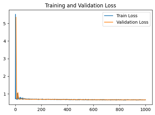
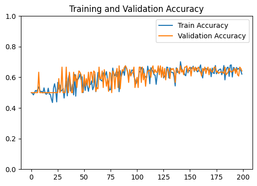
GNN Model | Test Accuracy = 0.6600 | F1 = 0.6316 |
We are going to compare our model to a Logistic Regression Baseline#
from sklearn.linear_model import LogisticRegression # Import the logistic regression model from sklearn

y_vals = labels.detach().cpu().numpy() # Get the labels as numpy arrays
input_data = g.ndata['feat'].detach().cpu().numpy() # Get the input features as numpy arrays

glmnet = LogisticRegression(penalty='l1' , solver='saga', max_iter = 1000 ) # Create a logistic regression model with L1 regularization
glmnet.fit(input_data[train_index] , y_vals[train_index][: , 0]) # Fit the logistic regression model
glmnet_acc = glmnet.score(input_data[test_index] , y_vals[test_index][: , 0]) # Get the accuracy of the logistic regression model on the test set
print(f'Baseline Logistic Regression ACC : {glmnet_acc}') # Print the accuracy of the logistic regression model
Baseline Logistic Regression ACC : 0.7625
/home/bryan/.conda/envs/bryanISMB/lib/python3.8/site-packages/sklearn/linear_model/_sag.py:350: ConvergenceWarning: The max_iter was reached which means the coef_ did not converge
  warnings.warn(
Our model does not outperform a simple linear regression model. This suggests that the gloabal relationships in the input data are stronger than the local relationships of our network
i.e. The local structure enforced by our network is less informative that learning from all features at once
In the next part, we will exhibit the predictive power of informative local structure by making a more informative network created from more than one modality