Part 2 - Patient Similarity Networks (PSNs)

Table of Contents

Part 2.

10. Patient Similarity Network Construction

11. DNA Methylation Network Analysis

# standard libraries
import os
import pickle

# scientific and data manipulation libraries
import numpy as np
import pandas as pd
from scipy import stats
from sklearn.feature_selection import mutual_info_regression
from astropy.stats import median_absolute_deviation
import mygene
import astropy

# graph and network libraries
import networkx as nx

# visualization libraries
import matplotlib.pyplot as plt
import seaborn as sns
import plotly.graph_objects as go
import plotly.io as pio
from IPython.display import Image
from IPython.display import display

import warnings
warnings.filterwarnings('ignore')

# import custom functions from the previous notebook
import sys
sys.path.insert(0 , '/tutorial/')
from functions import *

10. Patient Similarity Network (PSN)

• Based on the same expression matrix we can create a patient similarity network.

• Transposing the matrix will switch the rows and columns,

• meaning that patients will become the columns instead of genes

• By doing this, you can compute the correlation (or similarity) between patients based on their gene expression profiles,

• and then create a network where nodes represent patients and edges represent similarities.

# main data directories for the project

raw_data_dir = '/data/raw'
intermediate_data_dir = '/data/intermediate'

# read in os.path.join(intermediate_data_dir,"expression_data_filtered.csv")
df_renamed = pd.read_csv(os.path.join(intermediate_data_dir,
                                      "expression_data_filtered.csv"),
                                      index_col=0)

'''
#################################################
                YOUR CODE HERE
#################################################

We will now transpose the df_renamed df so that the rows represent the genes and the columns represent the patients.
Let's call the transposed df patient_gene_matrix.

'''

patient_gene_matrix = df_renamed.T

patient_gene_matrix

	TCGA-38-7271	TCGA-55-7914	TCGA-95-7043	TCGA-73-4658	TCGA-86-8076	TCGA-55-7726	TCGA-44-6147	TCGA-50-5932	TCGA-44-2661	TCGA-86-7954	...	TCGA-97-A4M7	TCGA-62-A46R	TCGA-50-5055	TCGA-38-4628	TCGA-86-7713	TCGA-86-8073	TCGA-MN-A4N4	TCGA-53-7626	TCGA-44-A47G	TCGA-55-6969
A2M	17.7492	14.8513	14.1691	16.7238	15.6783	14.7566	16.4368	15.5476	15.5478	15.1337	...	15.9553	13.9511	16.3097	14.3934	15.8254	16.3773	14.9411	16.7343	15.6622	14.8136
A2ML1	4.4411	4.4530	4.5026	3.1704	4.7422	6.0918	4.0602	3.0827	3.4608	3.6367	...	4.7076	2.4821	8.0810	3.3415	5.3379	4.0817	6.7210	5.2575	3.7345	4.3058
A4GALT	10.1862	8.9312	9.0834	9.1443	9.5150	11.4452	9.1462	7.3597	9.1602	8.9344	...	9.1019	8.6653	10.8837	8.6304	9.3827	9.4234	11.9107	9.5379	9.8660	9.7702
AACSP1	3.5845	3.6762	3.8623	2.4821	3.2271	2.4821	5.6614	3.0827	3.9428	4.7089	...	5.4947	3.0956	2.4821	3.7710	2.9397	6.6519	8.8283	2.4821	4.1045	6.8425
AADAC	9.6415	6.5685	5.5634	4.3206	7.2321	6.8821	8.1176	4.7935	11.7750	7.0644	...	9.0856	3.8162	5.6471	4.6785	4.6578	6.7641	3.4947	5.7120	6.2214	5.2016
...	...	...	...	...	...	...	...	...	...	...	...	...	...	...	...	...	...	...	...	...	...
ZSCAN23	5.7385	4.3796	5.6728	3.6533	5.0478	6.0489	5.8058	3.7897	4.3451	5.5259	...	4.7076	2.4821	4.6683	3.4697	4.3516	7.2074	6.9167	6.0927	5.3854	3.6792
ZSCAN31	9.0817	10.9565	10.8095	8.9874	9.5810	9.0185	10.2085	9.8803	11.0327	10.2707	...	9.2033	10.5020	8.8073	9.8672	10.6419	10.2410	9.4672	10.0507	7.4843	8.5268
ZSCAN4	3.2709	3.0918	2.4821	3.4468	3.0118	5.0894	5.5341	3.5082	5.4987	3.3645	...	4.4088	7.4937	4.3167	5.0907	6.7676	5.1126	3.3143	4.2816	4.4650	2.4821
ZWINT	9.2615	10.1334	10.9149	9.7828	8.6640	11.1212	9.0718	10.7305	9.0013	10.4268	...	9.7614	10.7593	9.7087	10.4729	10.9794	10.1390	10.0583	9.4627	9.5817	10.8228
ZYG11A	4.0073	8.3219	6.7593	3.4468	4.7844	5.0894	9.4014	4.7935	4.2748	7.1709	...	6.5412	7.1933	5.8778	7.3822	8.7596	8.2478	8.4566	7.4014	4.6804	8.6068

5338 rows × 498 columns

'''
#################################################
                YOUR CODE HERE
#################################################

We will now calculate the correlation matrix for the patient_gene_matrix using the Pearson correlation method.
Store the correlation matrix in a dictionary called patient_correlation_matrices with the key 'pearson'.
We don't have to do it, however if you want to calculate the correlation matrix using other methods,
you can do so and store them in the dictionary as well.

'''

# Dictionary to store different correlation matrices
patient_correlation_matrices = {}

# Pearson correlation
patient_correlation_matrices['pearson'] = patient_gene_matrix.corr(method='pearson')

'''
#################################################
                YOUR CODE HERE
#################################################

Create a graph from the correlation matrix using the create_graph_from_correlation function.
Set the threshold to 0.8.
Store the graph in a variable called patient_pearson_graph.

'''

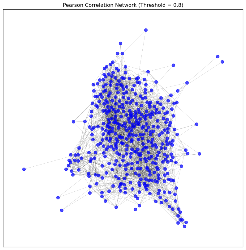
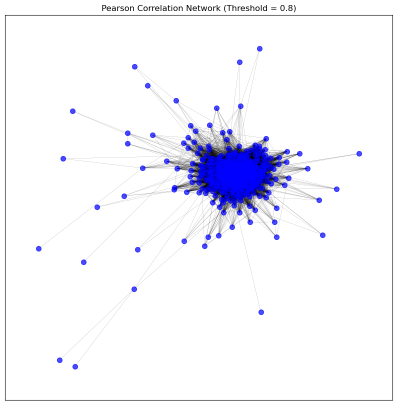
patient_pearson_graph = create_graph_from_correlation(patient_correlation_matrices['pearson'], threshold=0.8)

'''
#################################################
                YOUR CODE HERE
#################################################

Visualie the graph using the visualise_graph function.
Use appropriate title for the graph as the second argument.

'''
visualise_graph(patient_pearson_graph, title='Pearson Correlation Network (Threshold = 0.8)')

'''
#################################################
                YOUR CODE HERE
#################################################

Now use clean_graph function to clean the graph called patient_pearson_graph_pruned.
Consider the following parameters:
- degree_threshold
- keep_largest_component

'''
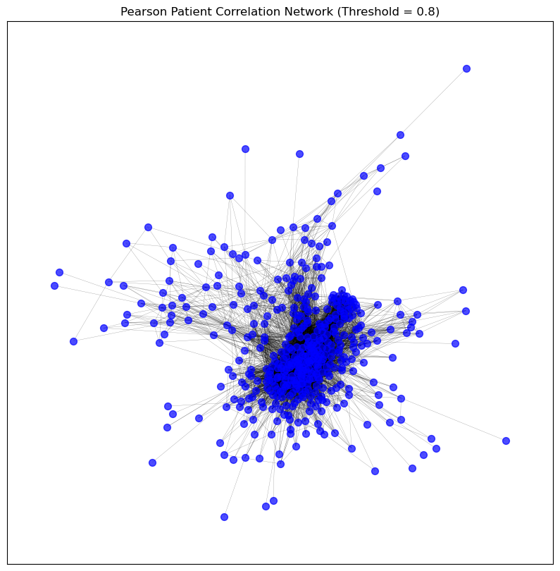
patient_pearson_graph_pruned = clean_graph(patient_pearson_graph,
                                    degree_threshold=1,
                                    keep_largest_component=True)

'''
#################################################
                YOUR CODE HERE
#################################################

Visualie the pruned graph using the visualise_graph function.
Use appropriate title for the graph as the second argument.

'''

visualise_graph(patient_pearson_graph_pruned,
                title='Pearson Patient Correlation Network (Threshold = 0.8)')

'''
#################################################
                YOUR CODE HERE
#################################################

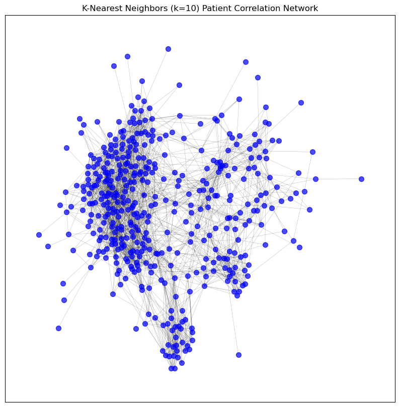
 Now do some sparsification of the graph using knn_sparsification function,
 call it patient_pearson_graph_pruned_knn.
 Set the k value to 10.               

'''

patient_pearson_graph_pruned_knn = knn_sparsification(patient_pearson_graph_pruned, k=10)

'''
#################################################
                YOUR CODE HERE
#################################################

Let's see some information about the graph using the print_graph_info function.
First, print the information about the patient_pearson_graph_pruned graph.
Use print("------------------------------------"), as a devide between the two graphs.
Then, print the information about the patient_pearson_graph_pruned_knn graph.            

'''

print_graph_info(patient_pearson_graph_pruned)
print("------------------------------------")
print_graph_info(patient_pearson_graph_pruned_knn)

Number of nodes: 434
Number of edges: 10373
Sample nodes: ['TCGA-38-7271', 'TCGA-55-7914', 'TCGA-73-4658', 'TCGA-86-8076', 'TCGA-55-7726', 'TCGA-44-6147', 'TCGA-50-5932', 'TCGA-44-2661', 'TCGA-86-7954', 'TCGA-73-4662']
Sample edges: [('TCGA-38-7271', 'TCGA-73-4658', {'weight': 0.8696511707884843}), ('TCGA-38-7271', 'TCGA-86-8076', {'weight': 0.8173779911639248}), ('TCGA-38-7271', 'TCGA-44-2661', {'weight': 0.8652686243802332}), ('TCGA-38-7271', 'TCGA-73-4662', {'weight': 0.8446135021161085}), ('TCGA-38-7271', 'TCGA-55-6986', {'weight': 0.833876175940164}), ('TCGA-38-7271', 'TCGA-49-6744', {'weight': 0.8919809060862212}), ('TCGA-38-7271', 'TCGA-69-7763', {'weight': 0.8374050473870502}), ('TCGA-38-7271', 'TCGA-44-6774', {'weight': 0.802120255633156}), ('TCGA-38-7271', 'TCGA-67-3774', {'weight': 0.8179727328277505}), ('TCGA-38-7271', 'TCGA-97-A4M2', {'weight': 0.8045412817214057})]
Graph type: undirected
No self-loops in the graph.
Graph density: 0.11039686678515555
Number of connected components: 1
Average clustering coefficient: 0.6049320008124544
------------------------------------
Number of nodes: 434
Number of edges: 2956
Sample nodes: ['TCGA-38-7271', 'TCGA-55-7914', 'TCGA-73-4658', 'TCGA-86-8076', 'TCGA-55-7726', 'TCGA-44-6147', 'TCGA-50-5932', 'TCGA-44-2661', 'TCGA-86-7954', 'TCGA-73-4662']
Sample edges: [('TCGA-38-7271', 'TCGA-53-7626', {'weight': 0.8932510135537189}), ('TCGA-38-7271', 'TCGA-49-6744', {'weight': 0.8919809060862212}), ('TCGA-38-7271', 'TCGA-78-8648', {'weight': 0.8857601471754217}), ('TCGA-38-7271', 'TCGA-86-8671', {'weight': 0.8825367028721114}), ('TCGA-38-7271', 'TCGA-50-5941', {'weight': 0.8814255405956031}), ('TCGA-38-7271', 'TCGA-55-7574', {'weight': 0.8799541588637929}), ('TCGA-38-7271', 'TCGA-97-7553', {'weight': 0.8775024097687647}), ('TCGA-38-7271', 'TCGA-50-5055', {'weight': 0.8726819735362153}), ('TCGA-38-7271', 'TCGA-50-5045', {'weight': 0.8723464616125998}), ('TCGA-38-7271', 'TCGA-73-4658', {'weight': 0.8696511707884843})]
Graph type: undirected
No self-loops in the graph.
Graph density: 0.03145986100616213
Number of connected components: 1
Average clustering coefficient: 0.3799854027043237

visualise_graph(patient_pearson_graph_pruned_knn, title='K-Nearest Neighbors (k=10) Patient Correlation Network')

11. DNA methylation PSN

In the second task, we are preparing an additional network for the same patients, this time based on DNA methylation data.

# Load the data using pickle from the ISMB_TCGA_DNAm.pkl file
with open(os.path.join(raw_data_dir,"ISMB_TCGA_DNAm.pkl") , 'rb') as file : 
    data = pd.read_pickle(file)

# Extract the methylation data from the dictionary similar to the previous data
meth_data = data["datExpr"]
meth_data

	cg23057992	cg16602369	cg20545544	cg04571941	cg23091104	cg11738485	cg17735539	cg12662576	cg10554839	cg08866780	...	cg04339424	cg01318691	cg27068965	cg23028848	cg21122529	cg22254072	cg10237911	cg09874052	cg27624178	cg02857943
TCGA-55-7914	0.039144	0.078881	0.032201	0.098520	0.971626	0.020020	0.929670	0.033325	0.043767	0.028051	...	0.053027	0.046047	0.951328	0.045767	0.048185	0.014262	0.034541	0.034967	0.041538	0.053116
TCGA-38-4631	0.954805	0.047287	0.027976	0.925794	0.144636	0.365842	0.156414	0.027917	0.047609	0.049901	...	0.048398	0.047221	0.939891	0.056141	0.047459	0.014548	0.056591	0.039086	0.044946	0.055473
TCGA-73-4658	0.966071	0.126549	0.030316	0.945166	0.976080	0.975638	0.942018	0.066659	0.052100	0.047054	...	0.040815	0.042040	0.951235	0.045477	0.074037	0.019053	0.029978	0.039345	0.060650	0.041385
TCGA-50-5932	0.965140	0.061194	0.935457	0.923421	0.965443	0.027598	0.040885	0.036178	0.045745	0.046439	...	0.057840	0.045106	0.948255	0.044558	0.039484	0.013837	0.037048	0.032503	0.058576	0.037666
TCGA-55-7576	0.958612	0.071607	0.027077	0.940574	0.976870	0.785073	0.953674	0.945107	0.056088	0.955472	...	0.046921	0.051442	0.954000	0.034352	0.031497	0.014924	0.035520	0.043547	0.056388	0.052208
...	...	...	...	...	...	...	...	...	...	...	...	...	...	...	...	...	...	...	...	...	...
TCGA-50-8457	0.960316	0.940219	0.046927	0.942980	0.977751	0.633731	0.940723	0.053398	0.059292	0.968875	...	0.047640	0.062680	0.954824	0.043137	0.048599	0.014066	0.031109	0.039247	0.035110	0.054273
TCGA-91-6840	0.964250	0.921250	0.957943	0.958416	0.981439	0.278432	0.968525	0.032143	0.083996	0.037912	...	0.045197	0.066271	0.963420	0.047621	0.060854	0.015823	0.045674	0.040006	0.052008	0.040826
TCGA-86-8280	0.948855	0.942925	0.958506	0.945667	0.970511	0.544447	0.921924	0.939427	0.082121	0.045036	...	0.062367	0.058898	0.954355	0.045702	0.048930	0.019321	0.039341	0.036627	0.054269	0.056795
TCGA-95-A4VK	0.037255	0.050940	0.036565	0.098237	0.976780	0.683394	0.960073	0.025232	0.062487	0.026908	...	0.056248	0.053591	0.947020	0.035344	0.057783	0.010943	0.051868	0.035566	0.044910	0.042269
TCGA-55-6969	0.945954	0.068404	0.923325	0.930684	0.962295	0.037952	0.153943	0.033980	0.056811	0.050211	...	0.048765	0.061228	0.930596	0.056050	0.061802	0.017861	0.044229	0.054682	0.045090	0.064186

459 rows × 300000 columns

# load the data from the pickle file ISMB_TCGA_GE.pkl and call it GE_data
with open(os.path.join(raw_data_dir,"ISMB_TCGA_GE.pkl"), 'rb') as file:
    GE_data = pickle.load(file)

# A reminder about the structure of the GE_data, we can get a list of the patients using the following code
GE_data["datMeta"]["patient"].to_list()

['TCGA-38-7271',
 'TCGA-55-7914',
 'TCGA-95-7043',
 'TCGA-73-4658',
 'TCGA-86-8076',
 'TCGA-55-7726',
 'TCGA-44-6147',
 'TCGA-50-5932',
 'TCGA-44-2661',
 'TCGA-86-7954',
 'TCGA-73-4662',
 'TCGA-44-7671',
 'TCGA-78-8660',
 'TCGA-62-A46P',
 'TCGA-55-6978',
 'TCGA-50-6592',
 'TCGA-38-4625',
 'TCGA-80-5611',
 'TCGA-86-8054',
 'TCGA-55-6986',
 'TCGA-L9-A5IP',
 'TCGA-69-7764',
 'TCGA-49-6744',
 'TCGA-75-5125',
 'TCGA-38-4626',
 'TCGA-69-7763',
 'TCGA-86-8279',
 'TCGA-93-8067',
 'TCGA-97-8179',
 'TCGA-55-A48Y',
 'TCGA-86-8055',
 'TCGA-91-6835',
 'TCGA-55-6982',
 'TCGA-55-A4DF',
 'TCGA-44-6774',
 'TCGA-50-5066',
 'TCGA-05-5423',
 'TCGA-67-3774',
 'TCGA-97-A4M2',
 'TCGA-95-7567',
 'TCGA-49-AAR0',
 'TCGA-44-2656',
 'TCGA-53-7813',
 'TCGA-O1-A52J',
 'TCGA-35-4122',
 'TCGA-55-8092',
 'TCGA-49-6761',
 'TCGA-49-4507',
 'TCGA-55-7816',
 'TCGA-78-7145',
 'TCGA-55-6983',
 'TCGA-53-7624',
 'TCGA-97-A4M3',
 'TCGA-50-5068',
 'TCGA-78-8648',
 'TCGA-44-6778',
 'TCGA-80-5608',
 'TCGA-86-8281',
 'TCGA-MP-A4T6',
 'TCGA-55-8085',
 'TCGA-62-8399',
 'TCGA-97-A4M5',
 'TCGA-97-7547',
 'TCGA-05-5429',
 'TCGA-55-7994',
 'TCGA-55-8094',
 'TCGA-05-4425',
 'TCGA-44-4112',
 'TCGA-49-6767',
 'TCGA-49-4490',
 'TCGA-MP-A4T9',
 'TCGA-50-5942',
 'TCGA-MP-A4SV',
 'TCGA-49-AAR4',
 'TCGA-05-4397',
 'TCGA-44-A47A',
 'TCGA-86-8359',
 'TCGA-78-7539',
 'TCGA-MP-A4T8',
 'TCGA-99-8032',
 'TCGA-50-6595',
 'TCGA-55-6968',
 'TCGA-44-8120',
 'TCGA-55-8302',
 'TCGA-99-8025',
 'TCGA-64-1679',
 'TCGA-95-8039',
 'TCGA-44-A479',
 'TCGA-44-6148',
 'TCGA-NJ-A55O',
 'TCGA-MP-A5C7',
 'TCGA-64-5778',
 'TCGA-55-6971',
 'TCGA-49-AARN',
 'TCGA-44-A47B',
 'TCGA-55-5899',
 'TCGA-49-AAQV',
 'TCGA-99-8028',
 'TCGA-75-6205',
 'TCGA-97-8552',
 'TCGA-50-8459',
 'TCGA-05-5425',
 'TCGA-78-7150',
 'TCGA-86-A4P7',
 'TCGA-49-4512',
 'TCGA-55-8206',
 'TCGA-55-8614',
 'TCGA-64-5815',
 'TCGA-L9-A50W',
 'TCGA-73-4675',
 'TCGA-55-7995',
 'TCGA-05-4433',
 'TCGA-55-7727',
 'TCGA-44-2668',
 'TCGA-44-A4SU',
 'TCGA-55-7907',
 'TCGA-69-7765',
 'TCGA-49-4487',
 'TCGA-44-2662',
 'TCGA-67-6216',
 'TCGA-55-7283',
 'TCGA-86-8280',
 'TCGA-91-6840',
 'TCGA-78-7154',
 'TCGA-49-4488',
 'TCGA-93-7348',
 'TCGA-62-A470',
 'TCGA-78-7147',
 'TCGA-50-5936',
 'TCGA-55-6984',
 'TCGA-50-5941',
 'TCGA-69-7978',
 'TCGA-78-7220',
 'TCGA-55-8616',
 'TCGA-44-A4SS',
 'TCGA-55-7570',
 'TCGA-78-7146',
 'TCGA-44-3398',
 'TCGA-05-5420',
 'TCGA-50-5072',
 'TCGA-05-4396',
 'TCGA-05-4405',
 'TCGA-50-5935',
 'TCGA-38-4629',
 'TCGA-55-8619',
 'TCGA-05-4410',
 'TCGA-73-4676',
 'TCGA-97-8172',
 'TCGA-44-7661',
 'TCGA-05-4384',
 'TCGA-44-2655',
 'TCGA-80-5607',
 'TCGA-67-3770',
 'TCGA-91-6836',
 'TCGA-95-7562',
 'TCGA-55-8511',
 'TCGA-44-6776',
 'TCGA-95-7948',
 'TCGA-91-7771',
 'TCGA-50-5944',
 'TCGA-MN-A4N5',
 'TCGA-73-4677',
 'TCGA-78-7540',
 'TCGA-91-6829',
 'TCGA-78-8640',
 'TCGA-62-8398',
 'TCGA-55-8512',
 'TCGA-83-5908',
 'TCGA-55-6987',
 'TCGA-93-A4JP',
 'TCGA-73-A9RS',
 'TCGA-L4-A4E5',
 'TCGA-86-8074',
 'TCGA-86-8358',
 'TCGA-78-7158',
 'TCGA-91-8497',
 'TCGA-49-AARO',
 'TCGA-78-7159',
 'TCGA-55-7227',
 'TCGA-86-7714',
 'TCGA-L9-A7SV',
 'TCGA-78-7143',
 'TCGA-91-8499',
 'TCGA-49-AAR3',
 'TCGA-55-8620',
 'TCGA-69-8255',
 'TCGA-75-6207',
 'TCGA-62-A46Y',
 'TCGA-NJ-A4YF',
 'TCGA-91-6830',
 'TCGA-62-8395',
 'TCGA-49-4486',
 'TCGA-44-6145',
 'TCGA-86-A4P8',
 'TCGA-78-7537',
 'TCGA-44-3919',
 'TCGA-35-4123',
 'TCGA-62-8394',
 'TCGA-69-7761',
 'TCGA-62-A46U',
 'TCGA-97-8547',
 'TCGA-97-7554',
 'TCGA-50-6673',
 'TCGA-95-7039',
 'TCGA-95-7944',
 'TCGA-55-8301',
 'TCGA-78-7152',
 'TCGA-05-4390',
 'TCGA-44-7659',
 'TCGA-97-7941',
 'TCGA-49-4514',
 'TCGA-55-A490',
 'TCGA-55-8508',
 'TCGA-MP-A4TE',
 'TCGA-97-A4M1',
 'TCGA-75-6206',
 'TCGA-86-8671',
 'TCGA-78-7160',
 'TCGA-64-1681',
 'TCGA-49-4494',
 'TCGA-50-5946',
 'TCGA-55-7913',
 'TCGA-44-6779',
 'TCGA-49-AARE',
 'TCGA-05-4403',
 'TCGA-99-AA5R',
 'TCGA-73-4659',
 'TCGA-50-8457',
 'TCGA-75-5147',
 'TCGA-55-8507',
 'TCGA-78-7536',
 'TCGA-95-A4VK',
 'TCGA-38-4627',
 'TCGA-67-6215',
 'TCGA-69-7973',
 'TCGA-05-5715',
 'TCGA-75-7030',
 'TCGA-44-2666',
 'TCGA-62-A472',
 'TCGA-55-6985',
 'TCGA-J2-A4AG',
 'TCGA-97-A4LX',
 'TCGA-55-6543',
 'TCGA-97-7938',
 'TCGA-35-3615',
 'TCGA-44-2657',
 'TCGA-55-8505',
 'TCGA-97-8175',
 'TCGA-49-4510',
 'TCGA-MP-A4TK',
 'TCGA-50-5044',
 'TCGA-49-AAR2',
 'TCGA-05-4250',
 'TCGA-97-7937',
 'TCGA-64-5774',
 'TCGA-86-8674',
 'TCGA-50-6590',
 'TCGA-64-5779',
 'TCGA-75-5146',
 'TCGA-44-6144',
 'TCGA-78-8662',
 'TCGA-55-7911',
 'TCGA-86-8585',
 'TCGA-38-A44F',
 'TCGA-64-1680',
 'TCGA-97-A4M6',
 'TCGA-75-6214',
 'TCGA-55-6980',
 'TCGA-97-7553',
 'TCGA-55-A48X',
 'TCGA-64-1677',
 'TCGA-73-7498',
 'TCGA-38-6178',
 'TCGA-44-7670',
 'TCGA-62-A471',
 'TCGA-49-4505',
 'TCGA-NJ-A7XG',
 'TCGA-55-6981',
 'TCGA-91-6848',
 'TCGA-55-8090',
 'TCGA-55-7725',
 'TCGA-55-8207',
 'TCGA-44-6146',
 'TCGA-05-4434',
 'TCGA-55-6979',
 'TCGA-05-4427',
 'TCGA-55-8615',
 'TCGA-50-5939',
 'TCGA-05-4418',
 'TCGA-67-6217',
 'TCGA-49-6745',
 'TCGA-55-1595',
 'TCGA-49-6742',
 'TCGA-05-4402',
 'TCGA-05-4382',
 'TCGA-55-7576',
 'TCGA-67-3773',
 'TCGA-78-7633',
 'TCGA-50-6597',
 'TCGA-44-2659',
 'TCGA-95-7947',
 'TCGA-55-7724',
 'TCGA-J2-A4AD',
 'TCGA-55-8091',
 'TCGA-55-1592',
 'TCGA-73-4670',
 'TCGA-55-1594',
 'TCGA-55-8621',
 'TCGA-50-5051',
 'TCGA-49-4501',
 'TCGA-J2-8194',
 'TCGA-44-8119',
 'TCGA-55-8203',
 'TCGA-97-8177',
 'TCGA-55-7573',
 'TCGA-55-8089',
 'TCGA-38-4630',
 'TCGA-78-7166',
 'TCGA-38-4631',
 'TCGA-55-1596',
 'TCGA-91-A4BD',
 'TCGA-67-3771',
 'TCGA-J2-8192',
 'TCGA-55-A48Z',
 'TCGA-97-8176',
 'TCGA-86-6851',
 'TCGA-50-5931',
 'TCGA-NJ-A4YI',
 'TCGA-97-7552',
 'TCGA-MP-A4T4',
 'TCGA-L4-A4E6',
 'TCGA-44-5643',
 'TCGA-MP-A4TD',
 'TCGA-05-4244',
 'TCGA-50-5930',
 'TCGA-44-6777',
 'TCGA-05-4430',
 'TCGA-05-4426',
 'TCGA-44-6775',
 'TCGA-05-4420',
 'TCGA-55-8506',
 'TCGA-44-7672',
 'TCGA-62-8402',
 'TCGA-86-8056',
 'TCGA-05-4422',
 'TCGA-75-7027',
 'TCGA-78-7535',
 'TCGA-50-8460',
 'TCGA-75-7031',
 'TCGA-L9-A444',
 'TCGA-73-4666',
 'TCGA-86-7953',
 'TCGA-86-A4D0',
 'TCGA-NJ-A4YQ',
 'TCGA-91-8496',
 'TCGA-67-3772',
 'TCGA-55-7281',
 'TCGA-05-4424',
 'TCGA-69-A59K',
 'TCGA-75-7025',
 'TCGA-55-8514',
 'TCGA-95-8494',
 'TCGA-05-4395',
 'TCGA-93-A4JQ',
 'TCGA-44-8117',
 'TCGA-55-8204',
 'TCGA-50-5933',
 'TCGA-MN-A4N1',
 'TCGA-55-7903',
 'TCGA-86-8669',
 'TCGA-55-6970',
 'TCGA-50-6594',
 'TCGA-86-8075',
 'TCGA-MP-A4TF',
 'TCGA-69-7760',
 'TCGA-78-7161',
 'TCGA-91-6849',
 'TCGA-99-8033',
 'TCGA-55-8205',
 'TCGA-55-8510',
 'TCGA-91-6828',
 'TCGA-50-5049',
 'TCGA-99-7458',
 'TCGA-49-AARR',
 'TCGA-MP-A4TC',
 'TCGA-49-AARQ',
 'TCGA-93-A4JN',
 'TCGA-95-A4VP',
 'TCGA-69-8453',
 'TCGA-55-8513',
 'TCGA-55-6975',
 'TCGA-86-8278',
 'TCGA-75-6203',
 'TCGA-49-6743',
 'TCGA-55-7574',
 'TCGA-78-8655',
 'TCGA-05-4389',
 'TCGA-86-7701',
 'TCGA-91-6831',
 'TCGA-55-7728',
 'TCGA-97-A4M0',
 'TCGA-50-6593',
 'TCGA-86-6562',
 'TCGA-62-A46S',
 'TCGA-86-A4JF',
 'TCGA-J2-A4AE',
 'TCGA-55-8087',
 'TCGA-78-7542',
 'TCGA-78-7148',
 'TCGA-55-A493',
 'TCGA-91-A4BC',
 'TCGA-05-4432',
 'TCGA-55-6712',
 'TCGA-4B-A93V',
 'TCGA-93-7347',
 'TCGA-86-8668',
 'TCGA-MP-A4TI',
 'TCGA-69-8254',
 'TCGA-64-1676',
 'TCGA-62-A46V',
 'TCGA-78-7167',
 'TCGA-55-7284',
 'TCGA-78-7162',
 'TCGA-75-6212',
 'TCGA-97-7546',
 'TCGA-44-5644',
 'TCGA-55-8299',
 'TCGA-75-6211',
 'TCGA-MP-A4SW',
 'TCGA-78-7149',
 'TCGA-S2-AA1A',
 'TCGA-95-A4VN',
 'TCGA-55-8096',
 'TCGA-05-4398',
 'TCGA-97-8171',
 'TCGA-55-A492',
 'TCGA-71-8520',
 'TCGA-44-3396',
 'TCGA-55-A57B',
 'TCGA-L9-A443',
 'TCGA-55-A4DG',
 'TCGA-67-4679',
 'TCGA-64-5781',
 'TCGA-93-A4JO',
 'TCGA-NJ-A4YP',
 'TCGA-69-7974',
 'TCGA-MP-A4T7',
 'TCGA-55-6642',
 'TCGA-49-AAR9',
 'TCGA-69-8253',
 'TCGA-05-4249',
 'TCGA-44-7669',
 'TCGA-71-6725',
 'TCGA-73-7499',
 'TCGA-MP-A4TH',
 'TCGA-55-8208',
 'TCGA-78-7156',
 'TCGA-75-5122',
 'TCGA-50-7109',
 'TCGA-NJ-A55R',
 'TCGA-53-A4EZ',
 'TCGA-NJ-A4YG',
 'TCGA-86-A456',
 'TCGA-38-4632',
 'TCGA-MP-A4TJ',
 'TCGA-97-8174',
 'TCGA-MP-A4SY',
 'TCGA-62-8397',
 'TCGA-L9-A8F4',
 'TCGA-75-5126',
 'TCGA-MP-A4TA',
 'TCGA-86-7711',
 'TCGA-50-5045',
 'TCGA-05-4417',
 'TCGA-44-7660',
 'TCGA-69-7979',
 'TCGA-55-A491',
 'TCGA-L9-A743',
 'TCGA-55-A494',
 'TCGA-44-7662',
 'TCGA-55-7910',
 'TCGA-69-7980',
 'TCGA-55-8097',
 'TCGA-73-4668',
 'TCGA-NJ-A55A',
 'TCGA-86-8672',
 'TCGA-86-8673',
 'TCGA-78-7153',
 'TCGA-97-A4M7',
 'TCGA-62-A46R',
 'TCGA-50-5055',
 'TCGA-38-4628',
 'TCGA-86-7713',
 'TCGA-86-8073',
 'TCGA-MN-A4N4',
 'TCGA-53-7626',
 'TCGA-44-A47G',
 'TCGA-55-6969']

We don’t want to include all CpG sites in our analysis, so we are using dataset from the EWAS Catalog that contains smoking related CpG sites.

smoking_df = pd.read_csv(os.path.join(raw_data_dir,"smoking.tsv"),
                          delimiter='\t')
smoking_df

	author	consortium	pmid	date	trait	efo	analysis	source	outcome	exposure	...	chrpos	chr	pos	gene	type	beta	se	p	details	study_id
0	Sikdar S	CHARGE	31536415	2019-09-19	Smoking	EFO_0009115, EFO_0006527, EFO_0004318	random effects meta-analysis	Table S2	DNA methylation	Smoking	...	chr2:233284934	2	233284934	-	Island	-0.08545	0.00131	0.000000	NaN	31536415_Sikdar-S_smoking_random_effects_meta-...
1	Sikdar S	CHARGE	31536415	2019-09-19	Smoking	EFO_0009115, EFO_0006527, EFO_0004318	random effects meta-analysis	Table S2	DNA methylation	Smoking	...	chr19:17000585	19	17000585	F2RL3	North shore	-0.07233	0.00129	0.000000	NaN	31536415_Sikdar-S_smoking_random_effects_meta-...
2	Sikdar S	CHARGE	31536415	2019-09-19	Smoking	EFO_0009115, EFO_0006527, EFO_0004318	random effects meta-analysis	Table S2	DNA methylation	Smoking	...	chr5:373378	5	373378	AHRR	North shore	-0.03138	0.00078	0.000000	NaN	31536415_Sikdar-S_smoking_random_effects_meta-...
3	Sikdar S	CHARGE	31536415	2019-09-19	Smoking	EFO_0009115, EFO_0006527, EFO_0004318	random effects meta-analysis	Table S2	DNA methylation	Smoking	...	chr2:233284402	2	233284402	-	Island	-0.07381	0.00132	0.000000	NaN	31536415_Sikdar-S_smoking_random_effects_meta-...
4	Sikdar S	CHARGE	31536415	2019-09-19	Smoking	EFO_0009115, EFO_0006527, EFO_0004318	random effects meta-analysis	Table S2	DNA methylation	Smoking	...	chr6:30720080	6	30720080	-	Open sea	-0.08558	0.00159	0.000000	NaN	31536415_Sikdar-S_smoking_random_effects_meta-...
...	...	...	...	...	...	...	...	...	...	...	...	...	...	...	...	...	...	...	...	...	...
40124	Domingo-Relloso A	Strong Heart Study	32484362	2020-06-02	Smoking	EFO_0004318, EFO_0005671, EFO_0006527	Former vs never	Table S3	DNA methylation	Smoking	...	chr6:32118295	6	32118295	PRRT1	Island	-0.05100	0.01310	0.000099	NaN	32484362_Domingo-Relloso-A_smoking_former_vs_n...
40125	Domingo-Relloso A	Strong Heart Study	32484362	2020-06-02	Smoking	EFO_0004318, EFO_0005671, EFO_0006527	Former vs never	Table S3	DNA methylation	Smoking	...	chr1:75599645	1	75599645	LHX8	North shore	-0.07300	0.01880	0.000099	NaN	32484362_Domingo-Relloso-A_smoking_former_vs_n...
40126	Domingo-Relloso A	Strong Heart Study	32484362	2020-06-02	Smoking	EFO_0004318, EFO_0005671, EFO_0006526	Pack years	Table S4	DNA methylation	Smoking	...	chr6:25992047	6	25992047	-	North shore	0.00268	0.00070	0.000099	NaN	32484362_Domingo-Relloso-A_smoking_pack_years
40127	Domingo-Relloso A	Strong Heart Study	32484362	2020-06-02	Smoking	EFO_0004318, EFO_0005671, EFO_0006526	Pack years	Table S4	DNA methylation	Smoking	...	chr10:33421027	10	33421027	-	Open sea	0.00112	0.00030	0.000099	NaN	32484362_Domingo-Relloso-A_smoking_pack_years
40128	Domingo-Relloso A	Strong Heart Study	32484362	2020-06-02	Smoking	EFO_0004318, EFO_0005671, EFO_0006526	Pack years	Table S4	DNA methylation	Smoking	...	chr15:41895799	15	41895799	-	Open sea	0.00109	0.00030	0.000099	NaN	32484362_Domingo-Relloso-A_smoking_pack_years

40129 rows × 31 columns

'''
#################################################
                YOUR CODE HERE
#################################################
1. Identify CpG sites that are commonly annotated in the smoking dataset
2. Filter the DNA methylation data to include only the common CpG sites identified in the previous step
3. Identify patients that are present in both the gene expression dataset and the methylation dataset
4. Filter the methylation data to include only the common patients and common CpG sites
5. Transpose the filtered methylation data matrix
'''

# Step 1: Count the occurrences of each unique value in the 'cpg' column using value_counts
cpg_counts = smoking_df['cpg'].value_counts()

# Step 2: Filter the counts to keep only those greater than 10
filtered_cpg_counts = cpg_counts[cpg_counts > 10]

# Step 3: Get the index of the filtered counts and convert it to a list
common_annotated_cpgs = filtered_cpg_counts.index.tolist()

# Step 4: Identify common CpG sites between the annotated list and the methylation dataset
cpgs = set(common_annotated_cpgs) & set(meth_data.columns)

# Step 5: Convert the cpgs set to a list
cpgs = list(cpgs)

# Step 6: Identify common patients between the gene expression and methylation datasets
# remember how to get the list of patients from dataset and to convert it to a list
common_patients = list(set(GE_data["datMeta"]["patient"].to_list()) & set(meth_data.index))

# Step 7: Filter the methylation data to include only the common patients and common CpG sites
meth_data_filt = meth_data.loc[common_patients, cpgs]

# Step 8: Transpose the filtered methylation data matrix and call it patient_meth_matrix
patient_meth_matrix = meth_data_filt.T

# let's inspect the patient_meth_matrix that we have created
patient_meth_matrix

	TCGA-75-6205	TCGA-97-7941	TCGA-97-7547	TCGA-95-7567	TCGA-95-7944	TCGA-69-7979	TCGA-55-7913	TCGA-55-8206	TCGA-55-6986	TCGA-64-5779	...	TCGA-91-8497	TCGA-MP-A4TC	TCGA-J2-8194	TCGA-75-7030	TCGA-50-5942	TCGA-86-7954	TCGA-78-7145	TCGA-62-A46R	TCGA-L9-A7SV	TCGA-86-8279
cg01731783	0.497444	0.396698	0.396081	0.403062	0.498713	0.411565	0.524197	0.400507	0.417326	0.518443	...	0.446258	0.568588	0.437242	0.452883	0.327272	0.467690	0.311361	0.421168	0.481429	0.429422
cg25949550	0.317716	0.140767	0.200784	0.483062	0.149553	0.259965	0.110951	0.144628	0.415628	0.165865	...	0.200756	0.206802	0.227245	0.205266	0.231608	0.159593	0.193704	0.331710	0.147767	0.137870
cg18316974	0.843950	0.579421	0.750254	0.879412	0.626643	0.192301	0.651054	0.810144	0.696567	0.545015	...	0.497423	0.680952	0.433783	0.515681	0.626869	0.515729	0.903988	0.860906	0.725199	0.371918
cg17372101	0.391085	0.602731	0.729051	0.349166	0.423132	0.378651	0.326185	0.575440	0.607495	0.251461	...	0.571380	0.254356	0.269948	0.499414	0.516246	0.357175	0.171478	0.269681	0.134351	0.192490
cg18146737	0.650549	0.442971	0.438343	0.735122	0.543430	0.184128	0.498125	0.386880	0.554262	0.494514	...	0.407518	0.578550	0.345746	0.446022	0.401742	0.427868	0.415197	0.753086	0.364550	0.419654
...	...	...	...	...	...	...	...	...	...	...	...	...	...	...	...	...	...	...	...	...	...
cg12803068	0.820755	0.664510	0.890526	0.899519	0.858862	0.817286	0.699223	0.796747	0.589624	0.692833	...	0.690219	0.766702	0.676125	0.582260	0.755870	0.683585	0.901678	0.796409	0.748843	0.822947
cg01207684	0.508975	0.187581	0.124399	0.299321	0.538336	0.128008	0.331944	0.184965	0.290967	0.246457	...	0.251051	0.352854	0.128596	0.280396	0.163345	0.287115	0.113246	0.338427	0.101977	0.099196
cg25305703	0.750465	0.858270	0.358668	0.315991	0.804947	0.682358	0.732886	0.861646	0.820864	0.488925	...	0.861702	0.685447	0.810510	0.811707	0.907132	0.818094	0.597665	0.818712	0.111031	0.356221
cg14580211	0.852855	0.760703	0.877694	0.837730	0.819975	0.874536	0.639945	0.844139	0.851723	0.789981	...	0.845984	0.648610	0.715354	0.746873	0.822599	0.887925	0.913990	0.834070	0.940591	0.797121
cg18446336	0.659491	0.637922	0.815690	0.795733	0.763106	0.813799	0.723343	0.828749	0.682581	0.751079	...	0.749783	0.687554	0.643351	0.789296	0.756348	0.712804	0.820558	0.760244	0.842471	0.862028

112 rows × 442 columns

We can finish our network following the previous steps using the functions we have created.

# Dictionary to store different correlation matrices
p_meth_correlation_matrices = {}

# Pearson correlation
p_meth_correlation_matrices['pearson'] = patient_meth_matrix.corr(method='pearson')

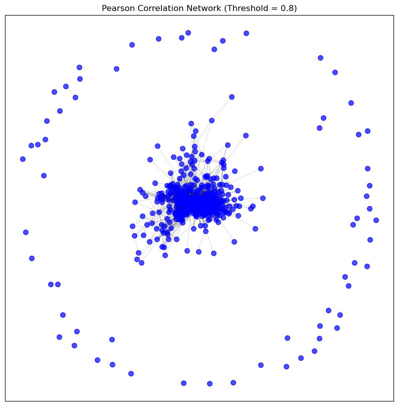
p_meth_pearson_graph = create_graph_from_correlation(p_meth_correlation_matrices['pearson'], threshold=0.8)
# Clean the graph by removing unconnected nodes
p_meth_pearson_graph_pruned = clean_graph(p_meth_pearson_graph,
                                    degree_threshold=1,
                                    keep_largest_component=True)

visualise_graph(p_meth_pearson_graph_pruned, title='Pearson Correlation Network (Threshold = 0.8)')

# sparseify the graph using knn_sparsification or any other method
p_meth_pearson_graph_pruned_knn = knn_sparsification(p_meth_pearson_graph_pruned, k=10)

# visualise the graph using the visualise_graph function
visualise_graph(p_meth_pearson_graph_pruned_knn, title='Pearson Correlation Network (Threshold = 0.8)')